Excel Formulas Cheat Sheet
The 30 Excel formulas everyone uses: SUM, IF, VLOOKUP, XLOOKUP, INDEX/MATCH, COUNTIF, dates and text — with examples.
Excel work slows down when you re-derive the same formula every time. This sheet collects the formulas office workers actually use daily, with a working example for each, so you can copy the pattern, change the cell references, and get on with the task.
Quick-Reference Table
The full data from this cheat sheet, right on the page.
| Formula | Example | What it does |
|---|---|---|
| SUM | =SUM(A1:A10) | Adds a range |
| AVERAGE | =AVERAGE(A1:A10) | Mean of a range |
| COUNT / COUNTA | =COUNT(A1:A10) | Counts numbers / non-empty cells |
| COUNTIF | =COUNTIF(A1:A10,"Yes") | Counts cells matching a condition |
| SUMIF | =SUMIF(A1:A10,"East",B1:B10) | Sums where a condition matches |
| IF | =IF(A1>=50,"Pass","Fail") | Returns one value if true, another if false |
| IFS | =IFS(A1>90,"A",A1>70,"B",TRUE,"C") | Multiple conditions without nesting |
| VLOOKUP | =VLOOKUP(A1,$D$1:$E$20,2,FALSE) | Looks up a value in the first column, returns a column to the right |
| XLOOKUP | =XLOOKUP(A1,D:D,E:E,"Not found") | Modern lookup — works left or right, built-in fallback |
| INDEX + MATCH | =INDEX(B:B,MATCH(A1,A:A,0)) | Flexible lookup, works in any direction |
| LEFT / RIGHT / MID | =LEFT(A1,3) | Extracts characters from text |
| TEXT | =TEXT(A1,"dd-mmm-yyyy") | Formats a value as text |
| CONCAT / TEXTJOIN | =TEXTJOIN(" ",TRUE,A1,B1) | Joins text with a delimiter |
| TRIM | =TRIM(A1) | Removes extra spaces |
| ROUND | =ROUND(A1,2) | Rounds to 2 decimal places |
| TODAY / NOW | =TODAY() | Current date / date and time |
| EOMONTH | =EOMONTH(A1,1) | Last day of a month offset |
| IFERROR | =IFERROR(A1/B1,"—") | Shows a friendly value instead of an error |
| AND / OR / NOT | =AND(A1>0,B1>0) | Combines logical tests |
| MAX / MIN | =MAX(A1:A10) | Largest / smallest value |
Printable Sheet Preview
High-Contrast Layout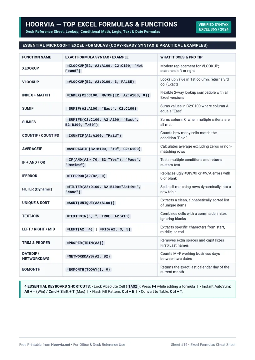
Download Your Free Printable Sheet
Download the printable PDF below. It is the same sheet shown in the preview above, ready to print on US Letter or A4 — open it and choose Print, with Scale set to Fit to Page.
💡 Pro Printing Tip: In your printer settings, set Scale to “Fit to Printable Area” and enable “Background Graphics” for color headers.
How to Print & Use This Chart
Print on US Letter or A4 and keep it beside your keyboard, or pin it to a cubicle wall where you can glance at it without switching windows. Use “Save as PDF” in the print dialog for a PDF copy in Letter or A4, and laminate it if your desk gets coffee rings — this is a sheet you will reach for daily in the first weeks of learning formulas. A second copy in a notebook is useful for remote work days, when the office wall chart is not beside you. Print it in colour if you can, but it remains readable in black and white because the structure is in the table, not the colour.
To use a formula, type it exactly as shown, then replace the example cell references with your own range — the pattern matters more than the letters. Lock a lookup table with dollar signs ($D$1:$E$20) before copying a formula down a column, or your range will drift row by row and return wrong results. Prefer XLOOKUP over VLOOKUP for new work: it handles lookups to the left, needs no column number, and has a built-in “not found” message. Wrap risky divisions and lookups in IFERROR so a spreadsheet shows a clean dash instead of #DIV/0! or #N/A to a manager. Test every new formula on a small sample first, check one result by hand, and only then copy it across thousands of rows — a fast wrong answer is worse than a slow right one.
Frequently Asked Questions (FAQs)
VLOOKUP or XLOOKUP — which should I learn?▼
XLOOKUP for new work: it is simpler, works in both directions, and handles missing values cleanly. Learn VLOOKUP too, because older files still use it.
Why does my copied formula give wrong results?▼
Usually a range drifted because it was not locked with $. Use $ before the column/row you want fixed when copying.
How do I avoid #N/A errors?▼
Wrap the lookup in IFERROR, e.g. =IFERROR(XLOOKUP(...),"Not found"), or check that the lookup value exactly matches, including spaces.
Can I use these in Google Sheets too?▼
Mostly yes — SUM, IF, COUNTIF, VLOOKUP and XLOOKUP work similarly, though some functions differ slightly. See the Google Sheets sheet on this site.